MBCAA Observatory

ASASSN-19cq: a gravitational microlensing event

Observed: 23 sessions in Feb-Mar 2019

Michel Bonnardeau
28 Feb, 1, 8, 10, 12, 17, 20, 27 Mar, 5, 7, 11 Apr 2019

Abstract

Photometric observations of this microlensing event are presented and interpreted.

Introduction

The discovery of the candidate microlensing event ASASSN-19cq was reported by Sokolovsky et al (2019), on Feb 12. I observed this event from Feb 13 until Mar 27, 2019.

Observations

The observations were carried out with a 203mm f/6.3 Schmidt-Cassegrain telescope, a V filter and a ST7E camera (KAF-401E CCD). The duration of each exposure is 200 s. A total of 471 valid images were obtained over 23 sessions.

For the differential aperture photometry, the comparison star is UCAC4 383-92972 (RA=17:46:48.98 DEC=-13:30:30.1) with an APASS magnitude V=12.227, and the check star is UCAC4 383-93080 (RA=17:46:58.07 DEC=-13:30:43.9).

The light curves:

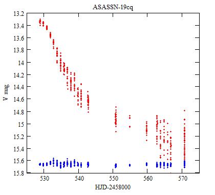
The individual measurements of ASASSN-19cq (red) and of the check star shifted by +3.1 mag (blue).

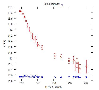
Each dot is the average of one session, and the error bars are ±1 standard deviation.

Analysis

The theory

The theory of the gravitational microlensing is explained in Wikipedia.

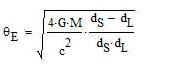
According to the GAIA DR2 catalog, the parallax to the lensed object is 0.0914±0.0389 mas so the distance is d_S=10941±4656 pc. Let be d_L the distance to the lensing object and M its mass. The Einstein angle is then:

The angular distance u(t) from the lensing object to the lensed star is, in unit of θ_E, with t_E the Einstein time:

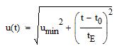
(u_min, the impact parameter, is the minimum distance, at t=t₀).

The amplification A of the flux from the lensed object is:

In the CMC14 catalog, the lensed star has the magnitudes r'=14.766, J=12.269, H=11.539 and K=11.325. Owing to the transformation formula of Bilir et al (2008) and Smith et al (2002) it can be computed that it has the magnitudes V₀=15.389 and g₀=16.217 in the V and g bands respectively (when not lensed).

The magnitude with the lensing effect is then:

V(t)=-2.5*log A(t)+V₀

A Monte Carlo fit

The V(t) function is fitted to the observations using a Monte Carlo method. There are 4 parameters to be adjusted: u_min, t₀, t_E and also V₀. V₀ needs to be adjusted because it is determined by transformations formulas, which are only approximate, and also to allow for a possible shift with the different photometry setups.

The 4 parameters are allowed to vary in the following ranges:
u_min around 0.15 ± 0.1
t₀ around the time of my first observation (2,458,528.71328 HJD) ± 1 day
t_E around 26 ± 10 day
V₀ around 15.389 ± 0.3 mag.

10⁶ sets of 4 parameters are taken randomly and, for each set, the quadratic sum of the residuals of V(t) from the observations, weighted with the uncertainties on the magnitudes, is computed. The set that gives the smallest residual is selected.

The process is repeated 10 times. The averages and the standard deviations of the selected sets of parameters are retained as the best fit to the observations.

Actually, this is repeated a number of times to be sure that the results are stable and that there is no degeneracy (i.e. different sets of parameters fitting the observations).

The results are:

u_min = 0.1715± 0.031
t₀ = 2,458,529.023± 0.046 HJD
t_E = 21.50± 0.58 days
V₀ = 15.269± 0.018 mag

and the resulting fit is shown in the figure below:

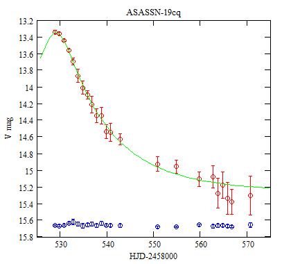
Green: the V(t) function.

With blending: Another way to fit the observations is to take into account the contribution of unresolved stars along the line of the sight to the overall received light. This blending effect (Nucita et al, 2018) may be accounting for by using the ratio of the source flux F_s to the total baseline flux F_s+F_blend:

f_s=F_s/(F_s+F_blend)

The magnitude with the lensing effect and the blending effect is then:

V_b(t)=-2.5*log[f_s*(A(t)-1)+1]+2.5*log(f_s)+V₀

A Monte Carlo fit is again performed, with a 5th parameter f_s, to be searched between 1 and 0.5. The results are, with 10 runs of 10⁷ trials:

u_min = 0.1317± 0.0057
t₀ = 2,458,529.088± 0.040 HJD
t_E = 26.81± 0.95 days
V₀ = 15.592± 0.053 mag
f_s = 0.776± 0.034

and the resulting fit is shown in the figures below:

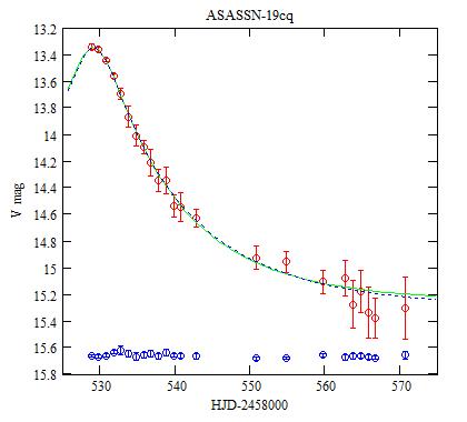
Dot blue: the V_b(t) function.

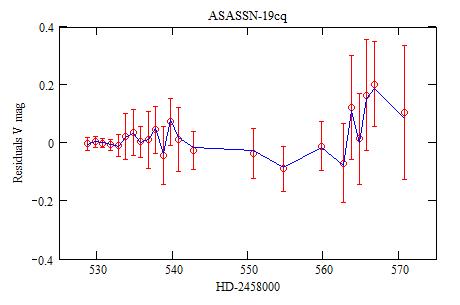
Red: residuals of the observations from the V(t) function, Blue: from the V_b(t) function.

About the microlens

The distance d_L to the lensing object, as a function of its mass M, for a given velocity v is:

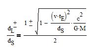
with the + for the lens being closer to the lensed object, and - for it closer to the observer.

The figure below gives d_L as a function of M for a velocity v=10km/s and for v=100km/s:

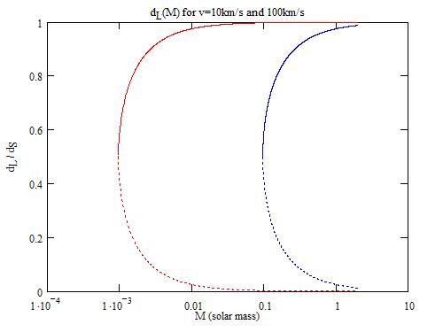
Continuous curves: d_L⁺, curves with dots: d_L^-. The 2 red curves on the left are for v=10km/s, the 2 blue curves on the right are for v=100km/s.

A Monte Carlo fit of the ASAS-SN data

The ASAS-SN data are available from https://asas-sn.osu.edu/. There are 76 measurements from HJD 2458519.15453 to 2458578.77813, obtained with a g filter. They are then fitted with the function:

g(t)=-2.5*log A(t)+g₀

owing to the Monte Carlo method, as above, except for the magnitude without the lens: g₀ around 16.217 ± 0.6 (not 0.3 as above, which appears to be too small here).

The results are:

u_min = 0.2169 ± 0.022
t₀ = 2,458,528.845 ± 0.022 HJD
t_E = 18.04 ± 0.27 days
g₀ = 15.711 ± 0.007 mag

With blending, the observations are fitted with the function, the same way as with my observations:

g_b(t)=-2.5*log[f_s*(A(t)-1)+1]+2.5*log(f_s)+g₀

This gives:

u_min = 0.151 ± 0.016
t₀ = 2,458,528.843 ± 0.019 HJD
t_E = 23.9 ± 1.9 days
g₀ = 16.15 ± 0.12 mag
f_s = 0.684 ± 0.070

The fit with the blending gives a value of g₀ very close to the one obtained from the CMC14 catalog.

The parameters obtained with blending are the same as (within the uncertainties) those obtained from my observations, also with blending. The blending factor is a bit stronger for ASAS-SN.

The resulting fits are shown in the figures below:

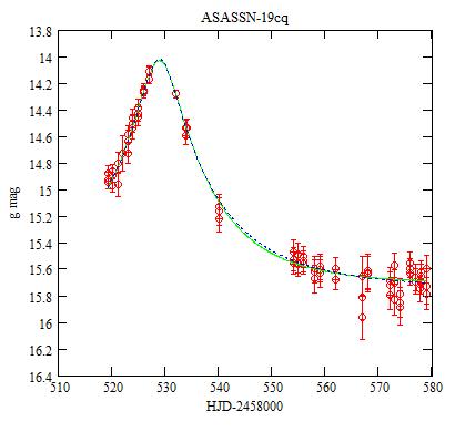
Red: ASAS measurements, Green: the g(t) function, Dot blue: the g_b(t) function.

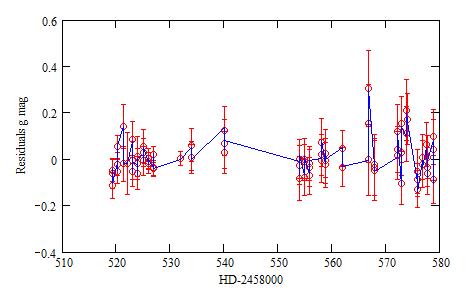
Red: the residuals from the g(t) function, Blue: from the g_b(t) function.

Conclusions

Both my observations and the ASAS-SN observations are fitted with the same gravitational microlens lightcurve. Furthermore, these observations are in different wavelength bands, which comforts the microlens interpretation.

The lensing object may have a mass in the range of 1/100 solar mass (a brown dwarf), anywhere along the line of sight. There is no evidence for a binary.

References

Bilir S. et al (2008) MNRAS 384 1178.
Nucita A.A. et al (2018) MNRAS 476 2962.
Smith J.A. et al (2002) AJ 123 2121.
Sokolovsky K.V. et al (2019) ATEL #12495.
Technical notes
Telescope and camera configuration.
Computer and software configuration.