MBCAA Observatory

GSC 318-805 / V551 Vir: a Blazhko star

Observed: 42 sessions from 2009 to 2015

Michel Bonnardeau
8 Dec 2015

Abstract

Photometric observations of the RR Lyrae star GSC 318-905/V551 Vir are presented and analyzed. They show a Blazhko modulation with a period of 53.9 days and evidence for irregularities. An animation showing the Blazhko modulation is presented.

Introduction

GSC 0318-0905 or ASAS J142306+0154.1 or NSVS 13340626 or V0551 Vir is an RRAB type pulsating star (RR Lyrae with a steep ascending light curve) with a pulsation period of 10.7 hr. It was reported by Wils et al (2006) as showing a Blazhko modulation with a period of 48 days. Apparently this is a little studied object, I report here photometric observations spanning 7 seasons.

Observations

The observations were carried out with a 203 mm Schmidt-Cassegrain telescope, Johnson V and B filters in a filter wheel (they may be used alternatively), and a SBIG ST7E camera (KAF401E CCD). The exposure durations were 200 s. The following table gives the numbers of useful images:

Season Nb of sessions Nb of V measurements Nb of B measurements

2009 3 72 68

2010 11 273 260

2011 6 166 158

2012 6 149 110

2013 5 259 0

2014 7 388 0

2015 4 284 0

Total 42 1591 596

For the differential photometry, the comparison star is GSC 318-984 with V=12.056 and B=13.182, computed from the CMC14 r' magnitude and the 2MASS magnitudes, owing to the transformations of Bilir et al (2008) and of Smith et al (2002).

An example of a light curve:

Green: GSC 318-905, Black: the check star. The error bars are the 1-sigma statistical uncertainties (computed as the q-sum of the uncertainties on the variable and of the comparison).

The B measurements are not analyzed here.

Analysis of the short period pulsation

The data are analyzed with the PERIOD04 software program (Lenz and Breger, 2005) which provides simultaneously sine-wave fitting and least-squares fitting algorithms. This yields the pulsation frequency:

F_P = 2.2378261 ± 4.2*10^-6 day^-1

or the pulsation period:

P_P = 0.4468622 ± 0.8*10^-6 day (0.07 s)

Owing to the PERIOD04 software program, the data are fitted with the following sine-wave function of the time t, with a number of harmonics of up to 4, above which they lost their significance:

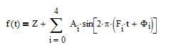
where t are the HJD - 2,454,000 and:

Z = 13.4625 +/- 0.0039

i F_i A_i Φ_i

0 F_P 0.3778 ± 0.0054 0.5022 ± 0.0024

1 F_P*2 0.1459 ± 0.0056 0.3653 ± 0.0060

2 F_P*3 0.0571 ± 0.0056 0.279 ± 0.015

3 F_P*4 0.0367 ± 0.0055 0.139 ± 0.023

4 F_P*5 0.0162 ± 0.0055 0.052 ± 0.055

The resulting phase plot and the residual of the observations from the f(t) function are shown in the figures below:

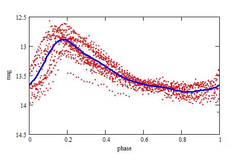
The red dots are the observations, the blue line is computed from the f(t) function. The phase origin is arbitrary.

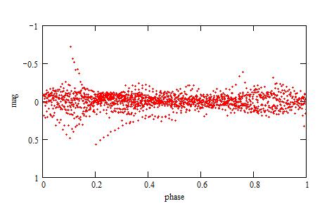
The differences between the observed magnitudes and the ones computed with the f(t) function.

The deviations around the f(t) function come from the Blazhko effect.

Analysis of the Blazhko modulation

The Blazhko modulation is expected to show up as side peaks around multiples of the pulsation frequency F_P in the Fourier spectrum (Breger & Kolenberg (2006), Szeidl & Jurcsik (2009)).

The PERIOD04 program is used to compute the Fourier spectrum of the residuals around the F_P frequency:
On the right side of F_P there are peaks at F_P+1/62, F_P+1/52 and F_P+1/45, and on the left side there are peaks (weaker than the ones on the right side) at F_P-1/62, F_P-1/52 and F_P-1/45.
Quite weaker, there are also peaks at F_P±2/62, F_P±2/52 and F_P±2/45.

The spectra of the residuals (observations - f(t)) around the frequency F_P. 45++ is the peak at F_P+2/45, 62- at F_P-1/62, and so on.

The spectra of the residuals around 2.F_P,3.F_P and 4.F_P also show peaks for ±1/62, ±1/52 and ±1/45.

The spectrum of the residuals around 5.F_P shows no clear signal.

These peaks are interpreted as a modulation with a period P_B around 52 days, and the signals at 62 and 45 days as due to the seasonal 1 year alias.

The data are then fitted with the following frequencies: F_P±1/P_B, F_P±2/P_B, 2.F_P±1/P_B, 3.F_P±1/P_B and 4.F_P±1/P_B. And the amplitudes and phases for the main pulsation are optimized again. The results are given in the table below:

i Interpretaion F_i A_i Φ_i

0 F_P F_P 0.3716 ± 0.0040 0.5067 ± 0.0018

1 2*F_P 2*F_P 0.1328 ± 0.0041 0.3601 ± 0.0050

3 3*F_P 3*F_P 0.0472 ± 0.0039 0.282 ± 0.013

3 4*F_P 4*F_P 0.0239 ± 0.0040 0.149 ± 0.028

4 5*F_P 5*F_P 0.0162 ± 0.0038 0.035 ± 0.034

5 F_P+1/P_P 2.2566168 ± 8.7E-6 0.0994 ± 0.0039 0.3890 ± 0.0063

6 F_P-1/P_P 2.218949 ± 1.2 E-5 0.0704 ± 0.0041 0.3770 ± 0.0087

7 F_P+2/P_P 2.274372 ± 1.9 E-5 0.0459 ± 0.0039 0.611 ± 0.013

8 F_P-2/P_P 2.200179 ± 3.6 E-5 0.0235 ± 0.0040 0.570 ± 0.027

9 2.F_P+1/P_P 4.495133 ± 4.3 E-5 0.0151 ± 0.0041 0.216 ± 0.029

10 2.F_P-1/P_P 4.456011 ± 2.5 E-5 0.0364 ± 0.0043 0.449 ± 0.018

11 3.F_P+1/P_P 6.732359 ± 1.3 E-5 0.0684 ± 0.0040 0.8914 ± 0.0091

12 3.F_P-1/P_P 6.694009 ± 4.5 E-5 0.0198 ± 0.0039 0.133 ± 0.032

13 4.F_P+1/P_P 8.970207 ± 2.1 E-5 0.0422 ± 0.0041 0.752± 0.015

14 4.F_P-1/P_P 8.931784 ± 4.1 E-5 0.0179 ± 0.0041 0.935 ± 0.031

In the above, there are 10 different evaluations of the Blazhko period (i=5 to 14). The average value and standard deviation are:

P_P = 52.5 ± 1.2 days

The observations may then be fitted with the function:

where ZB=13.4618 ± 0.0029

The residuals of the observations and of the fB(t) function are:

Comparison with the observations

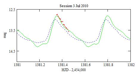
The 42 time-series are compared with the above fit. For most of them, the observations are found to be in good agreement with the fB(t) function. For example:

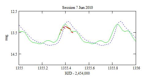
An example of a low amplitude Blazhko modulation which comes earlier than the short period pulsation. Red dots: the observations, Blue dotted line: the f(t) function, Green solid line: the fB(t) function.

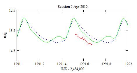
One month later the Blazhko modulation comes later and stronger than the short period pulsation.

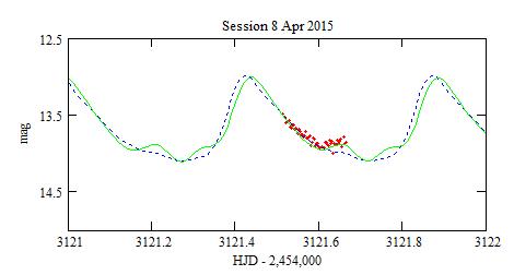
The Blazhko modulation is nearly in phase with the short period modulation with a bump.

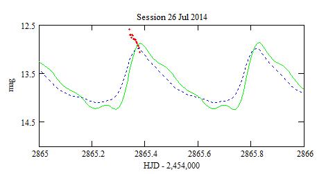
Less than a week later, the Blazhko modulation is much later, still with a bump.

However, sometimes the model does not fit the data. The 2 worst discrepancies are:

Refining the Blazhko period

Another iteration for the determination of the Blazhko period is done by scanning all the periods in the previous interval (52.5 ± 1.2),
regrouping the data in the same Blazhko phase interval (with an interval of 0.1 Blazhko period),
making a phase plot with the short period for each of these intervals,
summing the lengths of these phase plots.
The right Blazhko period is expected to give the smallest total length.

This is done for all the data except the 4 more discrepant time-series (the 2 shown above and 2 others). The resulting total length as the function of the Blazhko period is:

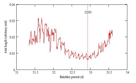
It has a sharp minimum at 52.93 ± 0.01 d.

The Blazhko modulation

By regrouping the data in the same Blazhko phase interval (of 0.1 Blazhko period), phase plots at different Blazhko phase can be made:

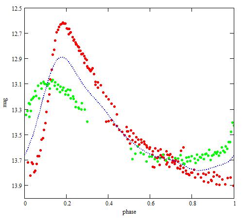
The red and green phase plots are separated in Blazhko phase by 0.5 Blazhko period. The Blue dotted line comes from the f(t) model.

To make the animation that follows better looking, 3 discrepant time-series were not taken into account (among the 4 that were not used for the derivation of the period). Furthermore 7 time-series were displaced from one phase interval to the adjacent one:

The Blazhko phase origin is arbitrary.

Conclusions

At the time of my observations, GSC 318-905 was found to have a Blazhko modulation with a period of 52.93 days, different from the 48 d reported by Wils et al (2006). However this Blazhko modulation cannot be described entirely by a periodic decomposition, it has irregularities. When compared with other RR Lyrae stars I observed, it is less regular than RV Cet but more than AR Ser (which has 2 Blazhko modulations).

References

Bilir S., Ak S., Karaali S., Cabrera-Lavers A., Chonis T.S. and Gaskell C.M. (2008) MNRAS 384 1178.
Breger M. and Kolenberg K. (2006) A&A 460 167.
Lenz P. and Breger M. (2005) Comm. Asteroseismology 146 53
Smith J.A., Tucker D.L., Kent S. et al (2002) AJ 123 2121.
Szeidl B. and Jurcsik J. (2009) Comm. Asteroseismology 160 17.
Wils P., Lloyd C. and Bernhard K. (2006) MNRAS 368 175.
Technical notes
Telescope and camera configuration.
Computer and software configuration.